A tool for automatic cortical shape identification for QCT scans.

This software is based on "Reinhold S. et al. (2019) [**An Analysis by Synthesis Approach for Automatic Vertebral Shape Identification in Clinical QCT**](https://doi.org/10.1007/978-3-030-12939-2_6). In: Brox T., Bruhn A., Fritz M. (eds) Pattern Recognition. GCPR 2018. Lecture Notes in Computer Science, vol 11269. Springer, Cham." (Full article, preprint)

Binary Releases

The current release is v1.2.2:

CortidQCT-v1.2.2-win64.zip Windows x64 binary release
CortidQCT-v1.2.2-macOS-Mojave.zip macOS Mojave binary release
CortidQCT-v1.2.2-x86_64-linux-gnu-ubuntu-18.04.tar.gz Ubuntu Linux 18.04 x86_64 binary release
CortidQCT-v1.2.2.mltbx MATLAB toolbox

Older releases can be found here.

Build from Source

The build instructions below are for *NIX (Unix/Linux/macOS) systems only. For Windows build, the configuration steps (1 to 4) should be the same, but the compilation step might be different, dependent on the compiler used.

C++ Library

Requirements

cmake version 3.9 or newer
A modern C++ compiler with C++17 support is required. These compilers are known to work:
- gcc: version 7.3 or later
- clang:
  - version 4.0 or later (with libc++ or stdlibc++-7.3 or later)
  - on Windows: version 7.0 with Visual Studio 2017 or later
- AppleClang: version 10.0 or later (Xcode 10, since macOS 10.4 Mojave)
- ~~MSVC++: version 14.1 or later (Visual Studio 2017 version 15.0 or later)~~ Due to a compiler bug MSVC 14.1 does currently not work

Building

CortidQCT uses the Hunter package manager to manage its dependencies. Therefore, it's not required to manually install any dependecies. Hunter builds and installs all dependencies automatically in the ${HOME}/.hunter directory. This can be changed by setting the HUNTER_ROOT environment variable.

It is strongly recommended to install CortidQCT to a custom location. For this, set the CortidQCT_ROOT environment to the desired path.

Clone the repository:
1 git clone htts://github.com/ithron/CortidQCT.git
Init the submodules:
1 cd CortidQCT
2 git submodule update --init
Create build directory
1 mkdir Build
2 cd build
Run cmake
1 cmake -DCMAKE_INSTALL_PREFIX=${CortidQCT_ROOT} -DCMAKE_BUILD_TYPE=Release ../
Run
1 make
installation
1 make install

MATLAB Toolbox

Requirements

MATLAB R2017b or later
Parallel Computing Toolbox
Statistics Toolbox
A CUDA compatible GPU
CUDA drivers

Installation

Navigate to the installation folder in MATLAB, then open matlab/CortidQCT.prj. This opens the toolbox packaging dialog. Click 'Package' and close the dialog. Double click the new file CortidQCT.mltbx to install the toolbox.

Usage

Using CortidQCT is a two step process. First a model for each different protocol must be generated using the MATLAB toolbox. After that, either the command line interface (CLI) tool, the C+++ library or the MATLAB interface can be used to identify the cortex using the generated model.

Model Creation


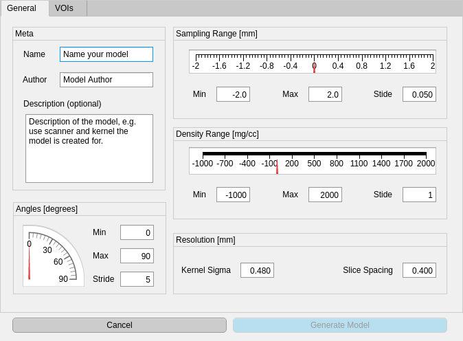
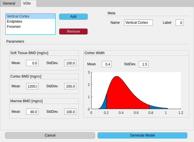
General model parameters dialog	Per VOI parameters dialog

In MATLAB run

1 CortidQCT.CreateModel

to start the model creation UI. On the first screen (general tab, see left screenshot above) meta and general information about the model can be entered. In the VOIs tab (see right screenshot above), per VOI prior parameters can be entered. Ensure that each VOI gets an unique label. Since the interpretation of the parameters of log-normally distributed cortex width parameter is not very intuituve, a plot of the current PDF is plotted in the bottom right. The red shaded region shows the 95% confidence interval.

After specifying all VOIs, click the Generate Model button start start the generation process. Depending on the hardware, this process may take a while. When the model generation completed, a green Save Model button will appear. Ensure to save the model before quitting the dialog.

Cortex Identification

You can either write your own program that uses the C++ library, use the built-in CLI tool or use the MATLAB interface that comes with the toolbox.

Command Line interface

After compilation the CortidQCT_CLI executable can be found in build/app. It requires at least three parameters:

A YAML configuration file
The input volume / scan
Path to the output mesh file
Optional: Path to a file where to write the per-vertex labels to

1 app/CortidQCT_CLI <configurationFile> <inputVolume> <outputMesh> [outputLabels]

C++ Library

The API Reference can be found here.

C Bindings

Available since Version v1.1.0. See the C-Bindings module in the API Reference for details. An example can be found in bindings/C/examples/cli.c.

Matlab Interface

Since version 1.2.0 CortidQCT also has MATLAB bindings, enabling the direct interaction with the library from within MATLAB.

An example implementation of the CLI interface can be found in examples/CortidQCT_cli.m:

 function [resultMesh, volume] = CortidQCT_cli(configFilename, volumeFilename, outputMeshFilename, varargin)
 %CORTIDQCT-CLI Identifies the cortical shape of the given volume and writes
 %the output to the given file
 
 import CortidQCT.lib.*;
 
 % Load volume
 volume = VoxelVolume.fromFile(volumeFilename);
 
 % Create MeshFitter using config file
 fitter = MeshFitter(configFilename);
 
 % fit
 result = fitter.fit(volume);
 
 % write output
 result.mesh.writeToFile(outputMeshFilename, varargin{:});
 
 % plot results
 volume.plot;
 hold on;
 h = result.mesh.plot;
 axis equal
 colormap gray
 
 h.FaceColor = 'g';
 h.FaceAlpha = 0.3;
 
 resultMesh = result.mesh;
 
 end

This function mimics the CLI application with additional visualization of the result:

Configuration File

The main purpose of the configuration file is to specify the reference mesh and the model file. Additionally some parameters can be customized. The configuration file must be in the YAML format.

Reference mesh

The following snippet defines a refernece mesh path/to/reference/mesh.coff consisting of a colored object file format mesh. Here each vertex color corresponds to a model label. The mapping is defined in the colorToLabelMap section. The custom mapping is supplied in the map section. Each element must be a two element list that contains a three element list and a single ineteger label: [[R, G, B], Label].

The origin: centerd parameter states that the centroid of the reference mesh should be moved into the center of the image, which is the default behaviour.

 referenceMesh:
   mesh: path/to/refernce/mesh.coff
   colorToLabelMap:
     type: custom
     map:
       - [[255, 0, 0], 1]¬
       - [[0, 255, 0], 0]¬
       - [[255, 255, 0], 2]¬
       - [[0, 0, 255], 3]¬
     undefinedLabel: 4
   origin: centered

If a relative path is given, it is interpreted as relative to the configuration file.

Measurement Model

The measurement model is specified by the path to the previously generated model file:

1 measurementModel: path/to/my/model.yml

If a relative path is given, it is interpreted as relative to the configuration file.

Optimization Parameters

There are several optional parameters that can be tuned:

 sigmaE: 5.4
 sigmaS: 2
 maxIterations: 100
 minNonDecreasing: 3
 decay: 0.1

sigmaE: Scale parameter of the ARAP shape prior energy term (defaults to 5.4). Note that due to a slightly different implementation, the parameter is not exactly like in the paper. If

is original parameter from the paper, then
$\tilde{sigma_E} := \sigma_E \sqrt{\exp(\sigma_E)}$
is the equivalent parameter for this implementation. So to reproduce the

= 2 from the paper, you have to set
$\tilde{sigma_E}$
= 5.4.
sigmaS: Displacement prior scale parameter, defaults to 2 (see paper).
maxIterations: Maximum number of iterations, defaults to 100.
minNonDecreasing: Minimum number of iterations before entering decay mode, defaults to 10
decay: Decay factor used in decay mode, defaults to 0.9.

Decay Mode

Since an approximate alternating optimization scheme is used, it might happen, that the optimizer oscillates between two solutions and never completely converges. To circumvent this oscillation, the mean absolute displacement is monitored. Everytime it doesn't decrease for at least minNonDecreasing iterations, the current sigmaS is multiplied by decay, resulting in a decay of step size over time, enforcing convergence.

Performance

This implementation is, opposed to the original prototype underlying the publication, highly optimized. While the original prototype required a few minutes for about 50 iterations, this implementation can make 50 iterations in about 20 seconds (on an Intel(R) Core(TM) i7-8700K CPU @ 3.70GHz).

The optimization time does of course depends on the size of the model and the scans.